Qeexo

TRY
BACK TO PRESS

ODR and FSR of Sensors

Dr. Rajen Bhatt and Josh Stone 28 May 2020

Qeexo’s AutoML enables Machine Learning and AI applications development for a range of sensors. A comprehensive list of sensors includes Accelerometer, Gyroscope, Magnetometer, Temperature, Pressure, Humidity, Microphone, Doppler Radar, Geophone, Colorimeter, Ambient light, and Proximity. In this article, we will discuss two very important configurable parameters that apply to many of these sensors, Output Data Rate (ODR) and Full-Scale Range (FSR).

Output Data Rate (ODR):

ODR (also known as “sampling rate”) is the rate at which a sensor obtains new measurements, or samples. ODR is measured in number of samples per second (Hz). Higher ODR configurations result in more samples per second.  Different sensor packages often come with multiple available ODRs, and it is typically up to the application developer to determine which ODR to use based on the needs of the application.

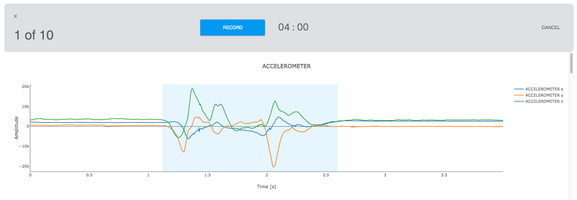
For example, accurately distinguishing between knocking and swiping on tabletop may require a higher ODR, in the range of several kHz (see Figure 1). This means that thousands of new samples are available every second, enabling the machine learning model to find the differences in rapidly changing vibration data. However, other applications such as distinguishing between walking, sitting, and running activities will likely operate very well in the range of 10-50 Hz, or tens of samples per second. Other types of scenarios, such as distinguishing between varying air gestures, fall between the previous two examples and will generally work well with ODRs in the range of 400-800 Hz.

Figure 1: Accelerometer impact data at 6.6 kHz (top) vs. 104 Hz (bottom)

Often, higher ODRs can improve model accuracy, since higher ODRs make more information available to the machine learning model. However, there are two major drawbacks to using higher ODR signals for embedded applications: memory constraints and power consumption.

Memory constraints need to be considered for ML models in embedded applications. On an embedded hardware platform, it is only possible to hold a relatively small number of samples in-memory, in addition to handling all of the processing required to prepare and run the machine learning model. Since this upper bound of samples is fixed, higher sensor ODRs have a lower maximum window size in terms of real time. For example, if a given hardware platform can only hold 1000 samples in memory at any given time, this represents approximately 2.5 seconds of 400 Hz data, while it only represents 1/3 of a second of 3.3 kHz data.

Power consumption also needs to be considered for embedded applications and will be higher for higher sampling rates. Generally, running machine learning on embedded devices means striking a good balance between performance of the machine learning algorithms and meeting power consumption constraints for the embedded application. This is an especially important consideration for models which will be deployed to devices running only on battery power. It is recommended to try building models with a few different ODRs and check the performance of the models.

Qeexo AutoML can build ML applications for all the available ODRs of sensors included in the supported hardware platforms. Accelerometers and gyroscopes generally have many different ODR options. Some industrial grade accelerometers can have ODRs as high as 26KHz, e.g., ~=26000 samples in one second. These accelerometers are capable of operating in industrial environments and are a great fit for machine monitoring applications on Qeexo AutoML.

Number of samples per second can vary depending on the hardware and firmware properties of the sensor module. Qeexo AutoML performs data quality checks, where it tests that the effective ODR matches the configured ODR of the sensors, among other things. We also recommend using Qeexo AutoML’s visualization tool to visually check the signal before training the ML models.

Full Scale Range (FSR):

Full Scale Range is associated with the range of values that can be measured for a given sensor and allows the application developer to trade-off measurement precision for larger ranges of detection. Two sensors that often have variable FSR settings are accelerometers and gyroscopes. Accelerometers measure the acceleration (rate of change of velocity of an object) in X, Y, and Z directions in the units of g (relative to the force of gravity). Gyroscopes measure angular velocity in Degrees per Second (DPS) in X, Y, and Z rotational directions.

Full scale range for accelerometers is generally programmable as ±2/±4/±8/±16 g, depending on the hardware platform. The smaller the range, the more sensitive the accelerometer will be to lower amplitude signals. For example, to measure small vibrations on a tabletop, using a FSR of 2g would provide more detailed data as it will be very sensitive to any minor accelerations, whereas using a 16g range might be more suitable to measure vibrations of somebody walking.

The DPS range for gyroscopes is generally programmable to ±125/±250/±500/±1000/±2000 depending on the hardware platform. The smaller the DPS range, the more sensitive the gyroscope will be to smaller angular motions. For example, to measure small angular motions for hand gestures used in a gaming application, using a smaller range would provide more detailed angular velocity data than using a 2000 DPS range, which might be more suitable to measure the angular motion of a fan.

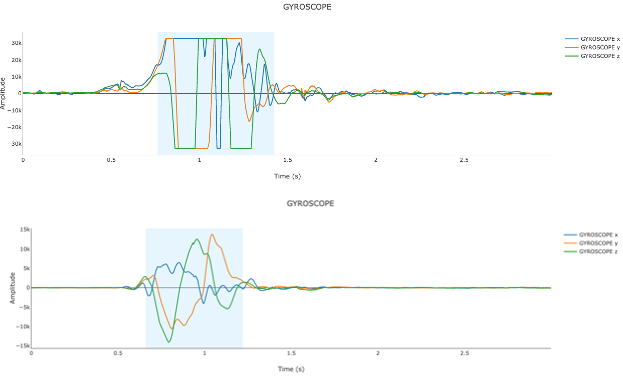
It is recommended to check for saturation of signals while working with FSR. If lower g and DPS are configured for accelerometer and gyroscope, but their actual measurements are higher than the configuration, their signals will saturate. Saturation happens because they cannot measure the desired physical quantities greater than their configuration, which would result in overflow. We recommend using Qeexo AutoML’s visualization tool to check for the saturation of the signals. Qeexo AutoML’s data quality check also checks for signal saturation and warns users when saturation is suspected.

Figure 2: Gyroscope motion gesture data at 125 DPS FSR (top) vs. 1000 DPS FSR (bottom)

BACK TO PRESS

Detecting Air Gestures with Qeexo AutoML

Josh Stone 26 May 2020

Project Description

We would like to build a machine learning model to distinguish between the following three classes:

– “X”
– “O”
– No gesture

This blog describes building the Air Gesture with Arduino Nano 33 BLE Sense. You can also build the same using any of the boards available on your Qeexo AutoML.

Sensor Configuration

For any sensor configuration, we need to consider three factors:

  • What type of data will capture the differences between our classes
  • What signal length will capture the differences between our classes
  • What range of sensor values will fully capture the range of our input

Based on these factors, we will select accelerometer and gyroscope sensors at 476 Hz for the air gesture problem. We will use +/- 8g and +/- 500 dps for the sensor FSRs.

These two sensors should be able to capture the type of data well, since they are motion sensors and our problem deals with differences in device motion.

Based on hardware memory constraints, we can only use 1024 samples per-channel on the Arduino Nano 33 BLE Sense, so an ODR of 476 Hz should allow us to have a signal length of multiple seconds to make each classification.

Finally, based on the fact that the device will be in motion, we will need a large range of possible sensor values. These larger values of FSR will prevent our sensors from saturation, even under scenarios of rapidly changing device position and speed.

Data Collection

For these three classes, we will need to use both types of AutoML data collection: event and continuous. To decide which type of data collection to use for each class, we need to consider the average time spent in a given class. If this time is 10 seconds or less, we should typically use event data collection. Otherwise, we’ll use continuous data collection.

Collecting continuous data

For the “no gesture” case, we will use continuous data collection, because we will often expect our final ML classifier output “no gesture” for long periods of time, sometimes minutes or even hours. We want our classifier to output “no gesture” for as long as the device is at rest. To collect continuous data, we will select Continuous, enter an appropriate class label, and enter an amount of time for an initial data collection. For now, we will collect 30 seconds to build an initial model – we can always collect more later if we find that performance isn’t as good as we’d like.

From there, we will press “Record” and go on to collect our “no gesture” data.

Collecting event data

Since the “X” and “O” letter gestures are discrete events, typically entering and exiting the class within a second or two, we will use event data collection.

To collect event data, we will select Event, enter an appropriate class label, and enter two additional values: a length per event, and a number of instances. For now, we will collect 10 instances to build an initial model. For length per event, we will select a number of seconds which will give you enough time to complete a full example of the given class. For example, since the “X” class takes 1-2 seconds typically, we will use a value of 3 or even 4 seconds to make sure we can complete the gesture in time.

From there, we will press “Record” and go on to collect our “X” and “O” letter gesture data.

Note: at the start and stop of each “event”, the device should be in an at-rest state. This will help AutoML to segment the incoming signal and determine where the actual event data occurred inside the collection window. This is why we should select a value for length per event which ensures we can start and stop the given event within the allotted time.

Here’s an example of a good event instance:

Note how the actual event is located fully within the collection window, and that AutoML is able to detect both the start and stop and highlight the event signal.

Here’s an example of a bad event instance:

When compared with the previous image, you can see how AutoML is not able to successfully find the full event range.

Model Training

After configuring our sensors and collecting our data, we are ready to build an initial model. We will select the data from our Training page and press “Start New Training”.

NOTE: The initial window that appears (step 1 of 4) is an optional “Group Labels” page. We can skip through this page for now, since we’ve only collected three classes of data, and we want to build a model which can distinguish between all three classes.

Sensor and Feature Selection

You will now be presented with Sensor and Feature Selection options (step 2 of 4). This section allows choosing a subset of recorded sensors and features to compute for each sensor, either automatically or manually. The automatic mode performs sensors and feature group selection fully automatically. Manual sensor selection can be combined with automatic feature selection or manual feature selection. For now, since this is our initial model, we will manually select both the recorded sensors, Accelerometer and Gyroscope and manually select all the feature groups available with both the sensors.

Configuring Inference Settings

The next step in building our initial model is configuring the inference settings (step 3 of 4). There is an option to have AutoML make these selections for you. If you want to use that option, please skip to the next section.

To manually configure the inference settings, we need to consider two things:

  • How long does the signal need to be for our model to make an informed decision?
  • How often does the class change for my problem?

In our case, our event signals last roughly 1-2 seconds. This timeframe should also be long enough to distinguish between either of our gestures and the “no gesture” class. Based on this reasoning, we will select 2000 ms as our instance length.

Since the current gesture class is user-controlled, and since we can move between classes quickly, we should select a fairly low value for the classification interval. A value of 500 ms should make classifications often enough to catch any changes between states.

Configuring Model Settings

The final step in building our initial model is configuring the model settings. There are a variety of options on this page, all of which control various aspects of the model-building process. You can select from among various models, chose to do hyperparameter optimization, or decide whether to generate learning curves.

For now, we will de-select all of the optional optimizations available at the top of the page and train a simple Logistic Regression model.

and train a simple Logistic Regression model. This model should be able to handle our small dataset well, as opposed to the deep learning models for which we might not have enough data and will hopefully find some simple patterns which can distinguish between these three classes.

Next you will see the real-time training progress of various steps of machine learning model training and results generation. Clicking on Training Results will show cross validation performance, library size, and latency of the model. Details will show many other results such as confusion matrix, ROC curves, and MCC matrix. You can flash the library using Live Test and after flashing is successful, your Arduino Nano 33 BLE Sense is ready to detect one of these three gestures.

BACK TO PRESS

Feature Selection Approaches: Part – I

Qifan He and Dr. Rajen Bhatt

In machine learning, the quality of feature selection strongly affects the quality of the trained model. Feature selections approaches differ depending on the type of machine learning problem, e.g., supervised learning or unsupervised learning. For supervised learning algorithms two most popular feature selection techniques are Wrapper-based and Model meta-transformer approach. For unsupervised learning algorithms, filter-based approaches are widely used.

In the part-I of this article, we will look into the wrapper-based feature selection approaches used for supervised learning problems.

Wrapper methods:

This approach keeps underlying ML algorithm in the loop with different subsets of features and sets the objective function quantifying the performance of the model, e.g., cross-validation score. Based on the strategy it adopts to iterate over different subsets of features, wrapper methods can further be categorized into exhaustive search, forward selection, backward selection, and k-best.

  1. Exhaustive search as its name suggests creates all the possible subsets of the actual feature sets and recommends the best subset according to the criterion. This approach is very time consuming as for p number of features it needs to evaluate 2p-1 combinations. For large p, this approach is almost impractical.
  2. Forward selection starts with zero features, evaluates each 1-feature model according to the defined criterion, and keeps the best performing feature at the root. Then makes 2-feature combination with the selected best and repeats the procedure until any further gain in the performance criterion cannot be achieved or all the features are exhausted. Fig. 1 explains the example run of forward selection algorithm with four features in the original set, X = {x1, x2, x3, x4}. Note the highlighted feature groups at each stage of the algorithm and algorithm termination with selected features {x2, x1, x4} because either the performance of {x2, x1, x4} is greater than or equal to {x2, x1, x4, x3}. For p number of features, this approach in the worst case evaluates p*(p+1)/2 combination of features instead of 2p-1 exhaustive combinations.
  3. Backward elimination first builds model with all the available features and recursively removes the least significant feature. The least significant feature can be identified by building models with all but one feature at a time and finding the drop in the performance. A feature which results in the performance drop of more than the threshold should be removed from the pool. The process continues until all the features with least significance are removed.
Fig. 1 Example Flow of Forward Selection Algorithm with Four Features

4. k-best approach is basically equivalent to running only the first stage of forward selection approach. It ranks each feature according to its performance on the defined criterion and can be cross-validation performance. Then it chooses the top k features, where k can be specified according the requirements on the memory, compute power, and latency.

Qeexo AutoML Feature Selection:

AutoML runs grouping-based forward selection wrappers method for feature selection to achieve the best model performance and smaller memory footprint libraries with low latency. To deal with continuously streaming data from multiple sensors at many different sampling rates, AutoML extracts hundreds of features from these streams. Some of these sensors are even multi-channel sensors, e.g., accelerometer, gyroscope, and magnetometer have three dimensional streams, colorimeter has four dimensional streams, etc. Multiple dimensions add to the complexity of feature space. To deal with such a large and complex feature space, AutoML categorizes feature space into several groups, for example, statistical-based, frequency-based, filter bank-based, etc. AutoML then runs forward feature selection algorithm on groups and recommends best feature groups.

AutoML expert mode also expose feature groups for each sensor to the user and then users can manually choose the feature groups. This approach allows users to rapidly iterate and trade off among various criteria library size, performance, and latency. In built visualizer projects the feature groups to 2-dimensional embedding space to visualize the classification properties of the selected group of features to guide the user selection.

For one-class problems, e.g., anomaly detection, Qeexo’s AutoML platform uses different methods to perform feature selection. These methods will be covered in Part-II.

BACK TO PRESS

Deep Learning in Qeexo AutoML Platform

Yanfei Chen and Dr. Rajen Bhatt

Deep learning (DL) has gradually become one of the most popular areas in artificial intelligence after the 1990s. Deep learning is a branch of machine learning and uses neural layers to build models. It combines low-level features and gradually forms abstract representation features to model the input data. Deep learning builds neural networks that simulates the human brain for analysis and learning. It mimics the mechanism of the human brain to interpret data, such as images, sounds, texts, and sensor readings.

According to the Universal Approximation Theorem [1], if a feedforward neural network has a linear output layer and at least one hidden layer with finite number of neurons and sigmoid activation function, it can approximate any continuous functions on a compact subset of ℝn with a sufficiently small error e > 0. This theorem is considered to be the theoretical basis of neural networks in deep learning.

The training process in deep learning is not particularly different from ordinary machine learning models. In deep learning, the objective is to find the weights of neurons or parameters of convolution filters in each layer, and this is done through predefined loss function, using gradient descent to continuously reduce the predefined loss, and strive to achieve the convergence. Backpropagation algorithm is the most common method for training neural networks. The algorithm will first calculate (and cache) the outputs of each layer according to the forward propagation, and then calculate the partial derivative of the loss function by applying chain rule with respect to each parameter in the way of traversing the graph backwards.

Deep neural networks, such as several common convolutional neural network models shown in the figure 1 [2], often have many parameters. Their parameters can often be in several thousands to millions depending on the application and size of the datasets presented for the learning. In the field of machine learning, the collection and labeling of training data is often a complicated and cumbersome process, which requires huge human and other resources. Thanks to Qeexo AutoML, the collection and labeling of the datasets is all integrated in the platform.

Tuning of deep learning model parameters is another challenge. For example, selecting the depth of the neural network, size of the convolution filters for each layer, what pooling to use, number of neurons in each layer, the learning rate, the optimization function, the batch size, number of training epochs, etc., often requires machine learning engineers to debug based on their knowledge and experience. This tuning process can be frustrating and time consuming. Deep learning is often very sensitive to model parameters, and the selection of model parameters will also affect the accuracy, size, and latency of the resulting model.

According to different learning tasks, commonly used models in deep learning include feedforward neural networks, convolutional neural networks, and recurrent neural networks. Qeexo AutoML platform for sensor data makes use of all these deep learning architectures for machine learning on micro-controllers. Due to memory, computation, and power consumption limitations on micro-controllers, Qeexo performs very sophisticated optimizations and model compressions on these architectures. Qeexo AutoML deep learning architectures does not require runtime interpreters when deployed on the microcontrollers. Libraries with no runtime make these models better suited for microcontrollers, they are light weight and has low latency.

Qeexo AutoML performs hyper-parameter tuning for deep learning models, saving time and effort of users dealing with this cumbersome process. Users also have a choice of configuring these model parameters themselves and if these parameters tend to generate models which are bigger than available memory size on the embedded devices, it performs automatic model reduction to make sure it fits on the device without sacrificing the model performance significantly.

Qeexo is one of the world’s first companies to run Deep Learning-based models from mobile phones. These models are light weight with latencies as low as 10 mSec. on mobile phone’s application processors. Qeexo’s AI engines are running on more than 300 Million mobile devices and growing rapidly. Today, Qeexo AutoML builds and deploys deep learning models on embedded targets using various sensor signals. Qeexo uses its proprietary model conversion technique to build light weight deep learning models on embedded microcontrollers. Additionally, Qeexo AutoML supports quantization-aware training of deep learning models. This type of training is aware of the fact that models are going to be quantized post-training and strives to retain the performance of the model despite quantization. Quantization can further reduce the model size while striving to maintain accuracy. This approach makes it possible to build bigger models when required to achieve high accuracy for certain applications.

References:

  1. Cybenko, G., “Approximations by superpositions of sigmoidal functions”Mathematics of Control, Signals, and Systems, 1989, 2(4), 303–314.
  2. LeCun, Yann, et. al. “Object recognition with gradient-based learning.” Shape, contour and grouping in computer vision. Springer, Berlin, Heidelberg, 1999. 319-345.