Qeexo

TRY
BACK TO PRESS

Sound Recognition with Qeexo AutoML

Zhongyu Ouyang and Dr. Geoffrey Newman 21 September 2020

Introduction

Sound Recognition is a technology based on traditional pattern recognition theories and signal analysis methods which is widely used in speech recognition, music recognition and many other research areas such as acoustical oceanography [1]. Generally, microphones are regarded as sufficient sensing modalities as input to machine learning methods within these fields. Microphones are capable of capturing information necessary for the variety of classification tasks that can be performed on lightweight devices. With this type of sensor, Qeexo AutoML provides a diverse feature stack, taking advantage of the physical properties of microphone data to extract information relevant to such classification tasks. This blog will show you how to perform sound recognition with Qeexo AutoML and explain some of the basics concepts of our feature stack.

AutoML Tutorial

Qeexo AutoML offers a general use user-friendly interface for engineers who wants to perform sound recognition, or any other classification task on embedded devices. The processes discussed in this blog are not specific to sound recognition, but are specifically applicable to it. To get started, navigate to the training page and select (or upload) the labeled training data that you want to use to build models for your embedded device. In the Sensor Selection page, you can select the desired sensor types, (in our sound recognition example we utilize the microphone sensor), to choose the collected data, as shown in Figure 1.

Figure 1: Sensor Selection Page

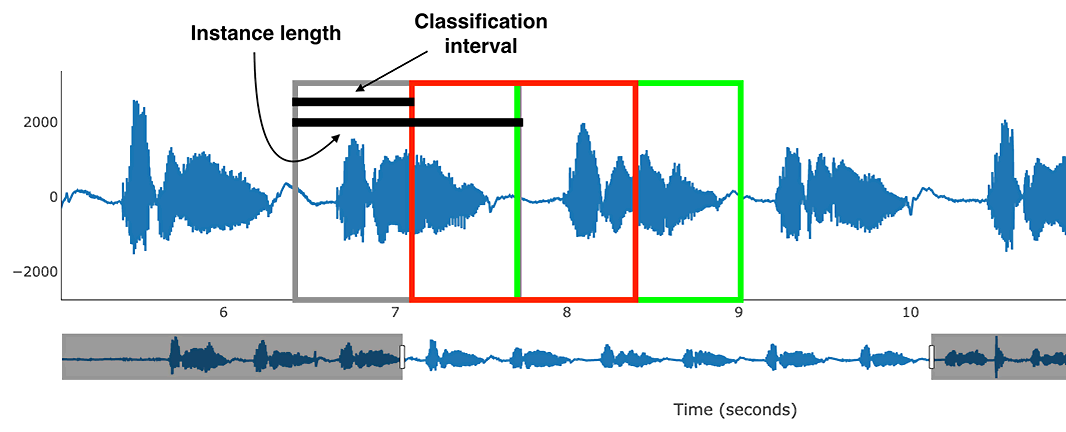
You are also provided with the option of automatic sensor and feature group selection, if you want to use additional sensor modalities or experiment with feature subgroups. If this is selected, Qeexo AutoML will automatically choose the sensor and feature groups that make the classes most distinct. In the Inference Settings page, you can manually set up the instance length and the classification interval, or let Qeexo AutoML determines them by selecting Determine Automatically, as shown in Figure 2.

Figure 2: Inference Settings Page

In the Model Settings page, you can pick the algorithm(s), choose whether to generate learning curve and/or perform hyperparameter tuning and click Start Training button to start. After the training is finished, a binary file will be generated and can be flashed to the device by clicking the Push to Hardware button. Once the process is finished, you can perform live tests on the model that was built, as shown in Figure 3.

Figure 3: Model Details Page

While the process is by design very straightforward, the details of some of the choices may appear ambiguous.
Other blog posts go into some detail on different aspects of the pipeline, but we will focus on some of the feature
choices applicable to sound recognition.

Sound Recognition Highlighted Features

Fast Fourier Transform (FFT)

Signals in the time domain are difficult for humans and computers alike to distinguish among similar sound sources. One of the most popular ways to transform raw sound data is the Fast Fourier Transform (FFT). Due to the constraints of embedded devices, the FFT is an efficient frequency decomposition technique. The process is described in Figure 4.

Figure 4: FFT process

For different classes, the signals differ in their magnitudes for a given frequency bin. E.g., in Figure 5, sounds generated with different instruments have different distributions of the magnitudes among the frequencies 0-800 Hz; even with differences present up to 2000 Hz.

Figure 5: FFT Features for Different Classes

The Qeexo AutoML training methods will take advantage of the increased class separability in this range to train the model through model training. Qeexo AutoML doesn’t just use all of the FFT coefficients as input in training the model, but actually aggregate the coefficients to create sophisticated features. The specific groupings can be hand-picked during the model selection process to accommodate implementation constraints. To select the features groups, simply check the box(es) in the manual feature selection page as shown in Figure 6.

Figure 6: Manual Feature Selection Page

Mel Frequency Cepstral Coefficients (MFCC)

Mel Frequency Cepstral Coefficients (MFCC) is also an important technique for sound recognition. Humans react differently to distinct ranges of frequencies. As a species, we are more capable of telling the difference in frequencies between a 50Hz and a 100 Hz signal, than that between 10050Hz and 10100 Hz. In other words, we are really bad at distinguishing high pitched sounds. Therefore, in situations where you want to replicate a task performed by humans, such as voice separation, the difference when the frequency is low is the most important. The value of the signal properties decreases with increasing frequency. Mel scale comes into place here, by assigning more importance to the low frequency content and less to the high frequency content. The formula for converting from frequency to Mel score is:

    \begin{align*} M(f) = 1125 * ln(1+f/700)\\ \end{align*}

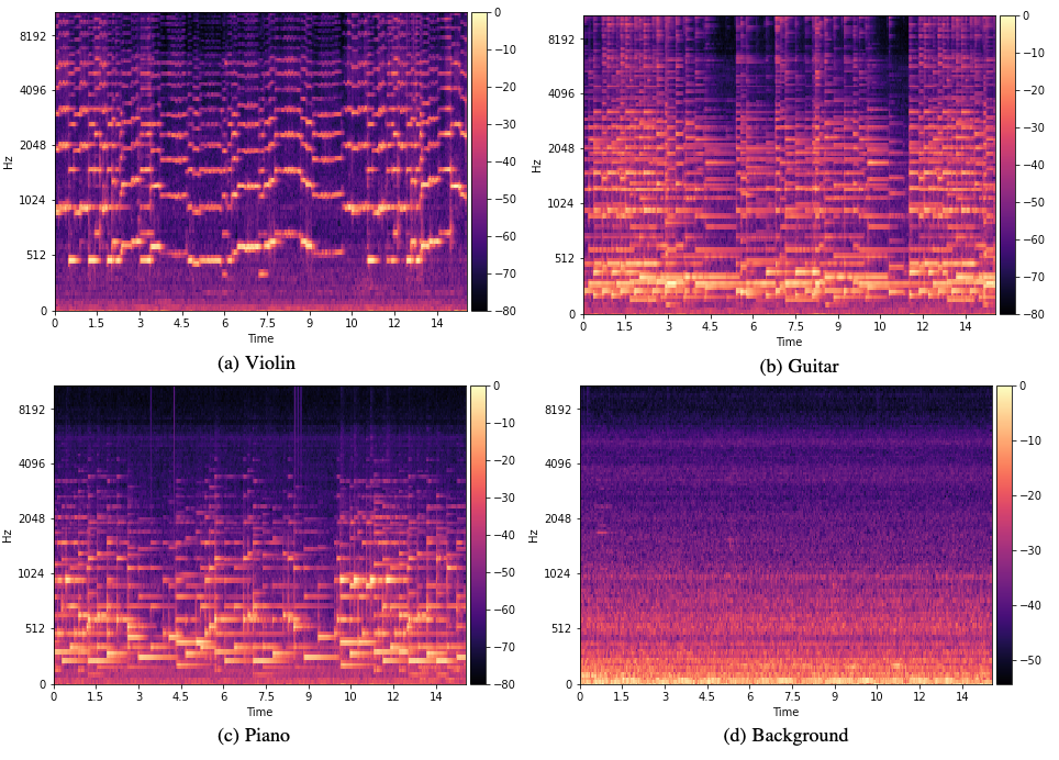
We build a filter bank containing many triangular filters and apply them to our FFT features to rescale the signals again and convert them to the corresponding Mel scales. In the Mel spectrograms shown in Figure 7, we can see that different classes’ Mel spectrograms appear to have many differences, making them ideal inputs for training a classifier.

Figure 7: Mel Spectrograms for Different Classes

Qeexo AutoML also provides features generated from the coefficients of MFCC. The feature groups can also be selected in the manual selection page shown in Figure 3. If desired, you can visualize the selected features through a UMAP plot by clicking the Visualize button shown in the Sensor Selection page and Feature Group Selection page.

Based on this discussion, it should be apparent that MFCC features will work well for tasks involving human speech. Depending on the task, it may be disadvantageous to include these MFCC features if it does not share similarities with human hearing. Qeexo AutoML performs automatic feature reduction, however, when automatic selection is enabled, so this does not need to be an active concern when training models. If the MFCC features are not highly separable for the task, assuming sufficient data is provided, they will be dropped from the final model during this process.

Conclusion

Qeexo AutoML not only provides model building functionality, but also present the details of the trained models. We provide evaluation metrics like confusion matrix, by-fold cross validation, ROC curve, and even support downloading the trained model to test it elsewhere. As mentioned earlier, we provide support for, but do not limit to microphone sensor usage for sound recognition. You are free to select any other provided sensors such as accelerometer and gyroscope. If these additional sensors don’t improve model performance, they won’t be included in the final device library, through the automated sensor selection process.

Bibliography

[1] Wikipedia: Sound Recognition,

https://en.wikipedia.org/wiki/Sound_recognition


BACK TO PRESS

Qeexo AutoML Enables Machine Learning on Arm Cortex-M0 and Cortex-M0+

Qeexo, Co. 09 September 2020

First company to build an automated ML platform for the Arm Cortex-M0 and Cortex-M0+ processor

MOUNTAIN VIEW, Calif. (PRWEB) September 09, 2020

Qeexo, developer of an automated machine learning (ML) platform that accelerates the deployment of tinyML at the edge, today announces that its Qeexo AutoML platform now supports machine learning on Arm® Cortex®-M0 and Cortex®-M0+ processors, which power devices including sensors and microcontrollers from companies such as Arduino, Renesas, STMicroelectronics, and Bosch Sensortec.

The Arm Cortex-M0 processor is the smallest Arm processor available, and the Cortex-M0+ processor builds on Cortex-M0 while further reducing energy consumption and increasing performance. Qeexo is the first company to automate adding machine learning to a processor of this size. The Cortex-M0 and Cortex-M0+ processors are designed for smart and connected embedded applications, and are ideal for use in simple, cost-sensitive devices due to the lower power-consumption and ability to extend the battery life of critical use cases such as activity trackers.

Machine learning models built with Qeexo AutoML are highly optimized and have an incredibly small memory footprint. Models are designed to run locally on embedded devices, ideal for ultra low-power, low-latency applications on MCUs and other highly constrained platforms.

“This integration delivers the advantages of data processing at the edge to even the smallest of devices,” said Sang Won Lee, co-founder and CEO of Qeexo. “Qeexo AutoML, combined with the accessibility of MCUs from companies such as Arduino, Renesas, STMicroelectronics, and Bosch Sensortec, greatly benefits application developers, who can now build smart hardware products with relative ease.”

The growing list of machine learning algorithms supported on Qeexo AutoML currently include: GBM, XGBoost, Random Forest, Logistic Regression, Decision Tree, SVM, CNN, RNN, CRNN, ANN, Local Outlier Factor, and Isolation Forest. Several hardware platforms from Arduino, Renesas, and STMicroelectronics work with Qeexo AutoML out-of-the-box.

Supporting Partner Quotes

Arm

“Today even the smallest devices can contain some layer of artificial intelligence and machine learning. The Cortex-M0 and Cortex-M0+ processors pack high performance with very low power consumption, and the added support of the Qeexo AutoML platform enables application developers to easily add intelligence to small devices such as wearables, making a world of one trillion intelligent devices a closer reality.”

— Steve Roddy, Vice President of Product Marketing, Machine Learning Group of Arm

Arduino

“Arduino is on a mission to make machine learning simple enough for anyone to use. We’re excited to partner with Qeexo AutoML to accelerate professional embedded ML development by guiding users to the optimal algorithms for their application. Combined with Arduino Nano 33 IoT, users can quickly create smart IoT sensors that can perform analytics at the edge, minimize communication, and maximize battery life.”

– Dominic Pajak, VP Business Development, Arduino

Bosch

“Bosch Sensortec and Qeexo are collaborating on machine learning solutions for smart sensors and sensor nodes. We are glad that Qeexo’s AutoML has added support for Cortex-M0 families, to which Bosch Sensortec’s smart sensors like BMF055 belongs. We are excited to see more applications made possible by combining the smart sensors from Bosch Sensortec and AutoML from Qeexo.”

– Marcellino Gemelli, Director of Global Business Development at Bosch Sensortec

Renesas

“Renesas and Qeexo collaborated on the design of a new RA-Ready sensor board: the RA6M3 ML Sensor Module. Equipped with various motion and environmental sensors and enhanced with Qeexo AutoML, this sensor module is the perfect reference platform for developing intelligent machine learning applications.”

– Kaushal Vora, Director of Strategic Partnerships & Global Ecosystem at Renesas

STMicroelectronics

“Qeexo AutoML recently added support for our STWIN industrial platform, which features embedded industrial-grade sensors and an ultra-low-power microcontroller for vibration analysis. By automating the development of ML solutions for advanced industrial IoT applications such as condition monitoring and predictive maintenance, Qeexo AutoML eases the usability of our products.”

– Pierrick Autret, Product Marketing Engineer at STMicroelectronics

###

About Qeexo
Qeexo is the first company to automate end-to-end machine learning for embedded edge devices (Cortex-M0-to-M4 class). Our one-click, fully-automated, Qeexo AutoML platform allows customers to leverage sensor data to rapidly build machine learning solutions for highly constrained environments with applications in industrial, IoT, wearables, mobile, automotive, and more.

Delivering high performance, solutions built with Qeexo AutoML are optimized to have ultra-low latency, ultra-low power consumption, and an incredibly small memory footprint. As billions of sensors collect data on every device imaginable, Qeexo can equip them with machine learning to discover knowledge, make predictions, and generate actionable insights.

Spun out of Carnegie Mellon University, Qeexo is venture-backed and headquartered in Mountain View, CA, with offices in Pittsburgh, Shanghai, and Beijing. To learn more, visit https://qeexo.com.

BACK TO PRESS

Inference Settings: Instance Length and Classification Interval

Xun (Jared) Liu, Dr. Rajen Bhatt, and Dr. Geoffrey Newman

Qeexo AutoML enables machine learning application developers to customize inference settings based on their use-case. These parameters are critical for achieving the best live performance of models on the embedded target. In this article, we will discuss the two parameters associated with the inference settings; instance length and classification interval.

Figure 1. Inference settings with microphone sensor (16000Hz) on Arduino

Instance Length

Instance length is the time period over which to make one prediction using raw sensor data. It is measured in milliseconds. According to the selected sensors and their ODRs, this time is then converted to the number of raw sensor data samples. These samples are used for computing features for training of ML models and also during on-device inference. If only one sensor is considered for the application, instance length is converted from milliseconds to number of samples using that sensor’s corresponding ODR. If there are multiple sensors with different ODRs, however, this conversion takes into consideration the sensor with the highest ODR. For other sensors, the number of samples is determined proportionally. Below are some examples for the Arduino sensor board with instance length of 500 milliseconds (0.5 seconds).

Setting 1: Microphone with ODR of 16000Hz.

Setting 2: Accelerometer and Gyroscope with 952Hz and microphone with 16000Hz.

For microphone,

For accelerometer and gyroscope,

How to Determine the Instance Length

Long instance length corresponds to a larger number of samples for featurization. According to Fourier Transform basic principles, more data points could yield finer frequency resolution, which captures an increased quantity of information from the signals. Therefore, it produces a greater number of features for the ML model training.

However, given the total time length, a long instance length would reduce the training dataset size. For example, if a signal of length L seconds is given and we divide that into segments of T seconds each, we get more segments if T is smaller and fewer if T is larger. For on-device live testing, larger T also implies more data needs to be collected at once to form a single prediction. Due to memory constraints of embedded devices, there will be limitations on the maximum instance length. Too small of an instance length can sometimes result in numerical instability of signal processing algorithms and may not capture sufficient discriminative information from the signals. For these reasons, AutoML restricts the minimum signal length to at least 64 samples.

Consider the following example for the microphone sensor (16000Hz) on Arduino. The instance length supported is at minimum 64 samples and at most 12000 samples. In milliseconds, this represents a range from 4 milliseconds to 750 milliseconds, as calculated here:

If multiple sensors (accelerometer & gyroscope; 952Hz ODR) are chosen, the range then becomes 4 to 1075 milliseconds.

Selecting the Best Instance Length

Qeexo AutoML supports automatically determining the instance length or setting it manually. The “Determine Automatically” option takes the minimum and maximum permissible values of instance length and finds the optimal value within this range. The optimization process tries to maximize the classification performance. It should be kept in mind for efficient model training that the optimization process takes longer to train models than manual selection.

Manual selection constrains the mininum and maximum permissible values. Any value within this range can be chosen for building the models. One way to estimate an instance length manually is visualizing the signal. As a general guideline, choose an instance length that is neither too short to miss part of the signal, nor too long that it could include unnecessary noise over multiple instances.

Instance length is a common parameter across all of the models, i.e., an instance length determined automatically or manually is applicable across all of the models.

Classification Interval (CI)

Classification interval refers to the time interval in milliseconds between any two classifications when live streaming sensor signals as illustrated in Fig. 3. It is a user defined parameter and accepts a value between 100 milliseconds (10 classifications in 1 second) and 3600 seconds (1 classification every 1 hour). Classification interval is not optimized even when selecting the “Determine Automatically” option.

Shorter intervals make predictions more frequent, but consume more power, while longer intervals save power, but can miss quick-burst live-streaming events when they occur between two consecutive classifications.

Figure 2. Instance length and classification interval

The detailed description of the Classification Interval is in this blog post.